Big edit: After sharing this I had the sudden panic (because, of course, this post has such a huge impact on the world) that I forgot to mention the gigantic assumption that I’m only looking at the sensible heat of the system, which is why I can treat the energy equations in terms of temperature (and not, say, enthalpy). That assumption makes the equations tractable but also puts a fairly significant limit to the application of the results. Namely if ice were in the cold bath (which is quite common), the latent heat of melting would keep the cold bath cold for much longer than this analysis predicts. Anyway, this analysis was done for the sake of curiosity so its results stand as they do.

At the new apartment, my brewing has gone outdoors to the back patio. The patio drains off onto the cars parked below the patio, so running an open loop of water through my wort chiller isn’t an option anymore. Not even to mention the ethics of dumping gallons of water during a drought.

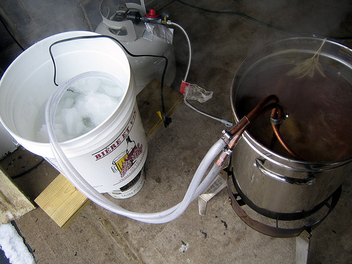
I went looking around for a submersible aquarium pump to run a closed-loop water cycle in a cooler – like the one shown in this image i jacked from some dude on flickr…

Of course I became curious about solving the energy balance for the temperatures of the wort as a function of time. It becomes interesting when you consider that the cold water flushes through the hot wort, and then warms up the cold bath as it dumps back into the reservoir. The curiosity is mostly academic and not really influencing a design as I see it. But … here goes.

Equations

In a really simplified sense, the hot wort and cold bath can be treated as coupled isothermal baths with one inlet/outlet of fluid. A schematic of the exchange is here:

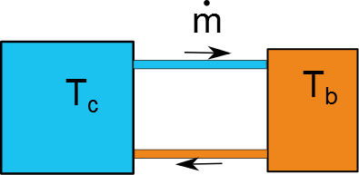
For this problem the cold fluid is all at $T_c$ whether its in the bath or in the transfer line. Same goes for the hot wort and hot end of the transfer line. Doing an open, transient energy balance on the two baths yields the simple coupled system of ODEs:

Obviously $\dot{m}$ is the mass flow pushed by the pump, and $m_b$ and $m_c$ are the masses of fluid sitting in the hot and cold baths, respectively. I’ll solve this by putting it into matrix form,

The vector-form of the simple ODE is solved in the same method as we would a classical first order ODE. Good detail can be found on this site. In other words, we can assume the solution is of some form (exponential) where the time constant in the exponential growth/decay comes from eigenvalues of the problem. For this system of equations, we find not only the eigenvalues but eigenvectors.

The two eigenvalues are $\lambda_1 = 0$ and $\lambda_2 = -(\dot{m}/m_b + \dot{m}/m_c)$. The corresponding eigen vectors are

and

Thus the general solution is

The initial conditions are left as just generic values for both baths. Plugging in those values at time $t=0$ to the general solution let’s us find the coefficients:

where $\Delta T_i$ is just the difference in temperatures of the two baths at the initial condition. I’ll define the ratio of hot-cold baths as a dimensionless parameter $\alpha$. When $\alpha < 1$, the hot bath is being cooled by a larger mass of cold water. Vice versa for $\alpha > 1$.

I want to clean up the solution a little so I’ll introduce another term, $\tau$ which I’ll consider as the time constant for the system. It’ll be defined as $\tau = \frac{m_b}{\dot{m}}$. This time can be thought of as how long it takes to move one hot bath’s worth of mass through the transfer lines. Finally, the solutions, when broken out of vector form, are

Short equation discussions

I’d like to actually pause to look at the solutions of the hot and cold bath temperatures. As a logic check, I want to see how the solutions look as $t\rightarrow \infty$; or in other words, steady state. For the hot bath we’re left with

For the simple case of when $\alpha = 1$ (aka equal sizes of hot and cold tanks), the final temperature of the hot reservoir is simply \(T_b = T_{b,i}/2 + T_{c,i}/2\): the average value of the initial temperatures. This is exactly what we should have expected so it’s good that it worked out.

I also would like to point out that this steady state temperature is not at all a function of the pump flowrate. It’s simply a mass-weighted average for temperature based on the sizes of my two tanks. The only place the flowrate does come in to play is in the exponential term – it dictates how quickly the system will reach the steady state / equilibrium.

Ok. With that little discussion out of the way, let’s look at some graphs…

Results

Background: I found a pump on Amazon that was $7 and ran at 80 gal/hr. I’ll assume that my wort is about 3 gallons. I’ll generally top off my fermenter with chilled water to hit 5 gallons so I aim for chilling the wort to only 80 F and then in the fermenter I can get pitching temperatures. These values will be used as guidlines for the computations.

I want to compare the temperatures of the two baths as the cold bath volume changes. Like, can 3 gal of frozen water drop 3 gal of boiling water to 80 F? (no). Or what size do I need in order to actually hit 80 F and how quickly will it reach it? The easiest way to solve this is with some simple scripting. The code is given in its entirety at the bottom.

Steady state final wort temperature

The first thing I want to plot are steady-state temperatures as a function of the mass-ratio, $\alpha = m_b/m_c$.

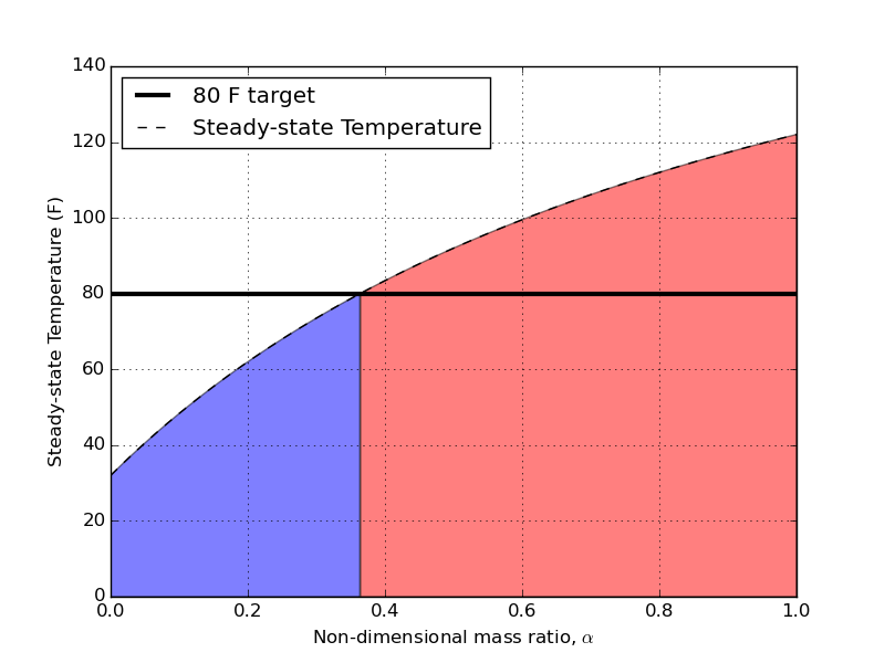
The shaded regions represent acceptable (blue) and unacceptable (red) mass ratios if we want to ever hit 80 F as the pitching temperature for our hot wort. The intersection of our target pitching temperature and the steady state value comes at $\alpha = 0.36$. This translates to a cold bath volume that is 2.8 times larger than the hot wort. For my example of having 3 gallons of hot wort, I’ll need 8.3 gallons of ice water when I begin to chill. That’s almost 9 gallons MINIMUM! That’s a remarkably large volume of water – considering the whole point of this was to try and conserve water during the cooling process. I think a future post will compare the total amounts of water consumed during open, closed, and mixed chilling.

Transient hot and cold temperatures with different volumes

Now that we know we need a minimum of $\alpha = 0.36$ in order to ever hit a pitching temperature, let’s see how the temperatures change in time for different $\alpha$ at a flowrate of 80 gph.

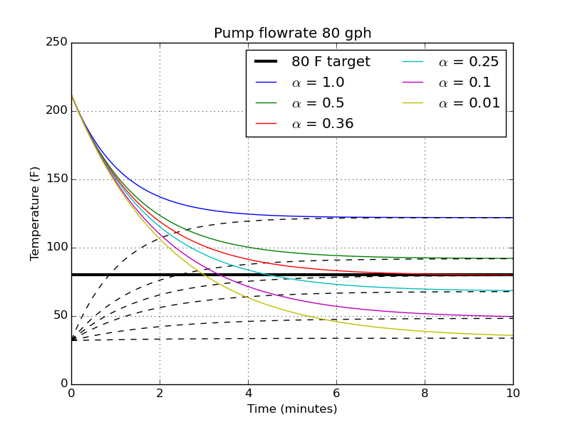
The upper and lower lines are the plots of hot and cold water temperatures, respectively. We see again that with $\alpha = 0.36$ we just barely will hit that 80 F target after sufficient time. With smaller volumes of cold water (larger $\alpha$), the cold bath raises up faster so the hot bath never has a chance to reach 80 F. As the cold volume increases ($\alpha < 0.36$), the target temperature is hit at earlier and earlier times.

For the next analysis, I want to take the ratio of $\alpha = 0.25$. It looks fast enough; it takes about 4 and a half minutes to hit 80 F. It also means if I have 3 gal of wort, I’ll need 12 gallons of ice water (that’s not too much, I guess?).

Transient hot and cold with different flowrates

The next logical step is to take my chosen mass ratio and find the temperature profiles for different flowrates.

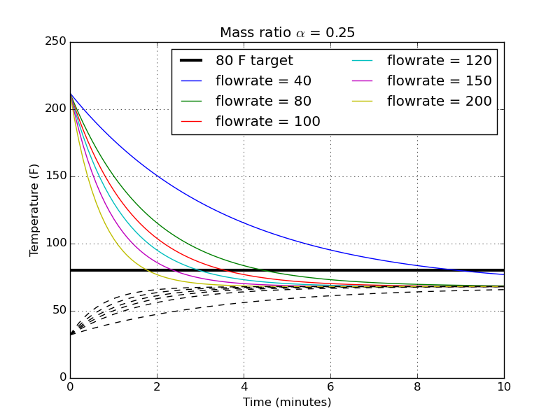
There’s a pretty dramatic difference in time between 40 gph and 80 gph, about 9 minutes for the slowest flowrate. You begin to then get diminishing returns for higher flowrate pumps. All the way to 200 gph, the time to hit my target temperature is only reduced to about 2 minutes from 4.5 minutes.

I must note, though, that I haven’t thought at all about how effective the physical wort chiller is that’s sitting in the hot liquid. I suspect that at the large flow rates, my assumption that the chilling water exits at the same temperature as the average temperature of the hot bath becomes less and less valid. That faster flow rate might be completely wasted if the efficiency of the chiller isn’t able to match it.

Conclusions…. kind of

Now… what does any of this have to do with buying a pump? Well, not much. The difference between an 80 gph pump and a 158 gph pump (at twice the price) would be hitting pitching temperature about a minute faster – given all the assumptions of my energy balance. Those flowrates are given by the pump description but I doubt I’d reach those values when its connected to the long copper coil of the wort chiller, and its concomitant pressure drop. I think the most important thing these equations highlight is how much more dependent the results are on the cold water volume than any aspect of the pump flowrate. If you don’t have ice in the system, you’re not going to get anywhere unless your cold water volume is almost 3 times larger than hot. That’s pretty interesting.

Code

I wrapped up the equations in some pert little code, reproduced here for posterity

import numpy as np
import matplotlib.pyplot as plt

def KtoF(T):
	# temperature converter for Kelvin to Farenheit
	return (T-273)*1.8+32

def StoM(t):
	# time converter for seconds to minutes
	return t/60

# Physical properties of the system
Qgph = 80
Q = Qgph * 0.00105150 # gal/hr to L/s
rho = 1000     		# water density 
Vb = 3*.00379  		# gal to m3 hot bath
mb = rho*Vb  		# mass of the wort
Tci = 273 			# K
Tbi = 373 			# K
DeltaTi = Tbi - Tci
t = np.linspace(0,600,100) # timespan

# Non-dimensional parameters
alphas = np.array([1, 0.5, 0.36, 0.25, 0.1, 0.01])
tau = mb/Q





# Analysis of steady-state~~~~~~~~~~~~~~~~~~~~~~~~~~~~~~~~~~~~~~~~~~~~~~~~~~~~~~~~~~~~~~~~
alphaArray = np.linspace(0, 1, 1000)
Tf = Tbi - DeltaTi/(1+alphaArray) 
Taim = np.zeros(len(alphaArray))+80 # the temperature we're aiming for (as an array with time)

TfGood = Tf[np.where(KtoF(Tf)<80)]
alphaGood = alphaArray[np.where(KtoF(Tf)<80)]
TfBad = Tf[np.where(KtoF(Tf)>80)]
alphaBad = alphaArray[np.where(KtoF(Tf)>80)]
alphaMin = alphaGood[-1]
print "Minimum necessary mass-ratio = " + str(round(alphaMin,2))

plt.figure(1)
plt.plot(alphaArray, Taim,'k',linewidth=3,label='80 F target')
plt.plot(alphaArray, KtoF(Tf), 'k--', label='Steady-state Temperature')
plt.fill_between(alphaGood, KtoF(TfGood), 0, facecolor='blue', alpha=0.5, label=r"Required $\alpha$")
plt.fill_between(alphaBad, KtoF(TfBad), 0, facecolor='red', alpha=0.5, label=r'Unacceptable $\alpha$')
plt.xlabel(r'Non-dimensional mass ratio, $\alpha$')
plt.ylabel("Steady-state Temperature (F)")
plt.legend(loc='best')
plt.grid()
# /Analysis of steady-state~~~~~~~~~~~~~~~~~~~~~~~~~~~~~~~~~~~~~~~~~~~~~~~~~~~~~~~~~~~~~~~



# Analysis of transient~~~~~~~~~~~~~~~~~~~~~~~~~~~~~~~~~~~~~~~~~~~~~~~~~~~~~~~~~~~~~~~~
Taim = np.zeros(len(t))+80 # the temperature we're aiming for (as an array with time)
# set up the figure
plt.figure(2)
plt.plot(StoM(t),Taim,'k',linewidth=3,label='80 F target')
plt.xlim([0,StoM(t[-1])])
plt.xlabel('Time (minutes)')
plt.ylabel("Temperature (F)")
plt.grid()

# looping over different cold water / hot water bath volumes
# to find the solution of temperature with time
# reminder: alpha = m_b / m_c
for alpha in alphas:
	gamma = DeltaTi/(1+alpha) # intermediate calc
	Tb = Tbi - (1 - np.exp(-(1 + alpha)*t/tau))*gamma
	Ti = Tbi - (1 + alpha*np.exp(-(1 + alpha)*t/tau))*gamma
	
	# plot the current temperature profiles
	plt.plot(StoM(t),KtoF(Tb), label=r'$\alpha$ = '+str(alpha))
	plt.plot(StoM(t),KtoF(Ti), 'k--')
plt.legend(loc='best', ncol=2)
plt.title('Pump flowrate %s gph'%(Qgph))
# /Analysis of transient~~~~~~~~~~~~~~~~~~~~~~~~~~~~~~~~~~~~~~~~~~~~~~~~~~~~~~~~~~~~~~~


# Analysis of flowrate~~~~~~~~~~~~~~~~~~~~~~~~~~~~~~~~~~~~~~~~~~~~~~~~~~~~~~~~~~~~~~~~
# set up the figure
plt.figure(3)
plt.plot(StoM(t),Taim,'k',linewidth=3,label='80 F target')
plt.xlim([0,StoM(t[-1])])
plt.xlabel('Time (minutes)')
plt.ylabel("Temperature (F)")
plt.grid()

Qgph = [40, 80, 100, 120, 150, 200]

alphaQ = 0.25
# looping over different flowrates
# to find the solution of temperature with time
for q in Qgph:
	Q = q
	q = Q * 0.00105150 # gal/hr to L/s
	tau = mb/q
	gamma = DeltaTi/(1+alphaQ) # intermediate calc
	Tb = Tbi - (1 - np.exp(-(1 + alphaQ)*t/tau))*gamma
	Ti = Tbi - (1 + alphaQ*np.exp(-(1 + alphaQ)*t/tau))*gamma
	
	# plot the current temperature profiles
	plt.plot(StoM(t),KtoF(Tb), label=r'flowrate = '+str(Q))
	plt.plot(StoM(t),KtoF(Ti), 'k--')
plt.legend(loc='best', ncol=2)
plt.title(r'Mass ratio $\alpha$ = %s'%(alphaQ))
# /Analysis of flowrate~~~~~~~~~~~~~~~~~~~~~~~~~~~~~~~~~~~~~~~~~~~~~~~~~~~~~~~~~~~~~~~

plt.show()

• ← Previous Post
• Next Post →